Symmetric Matrices and Orthogonal Diagonalization

Many algorithms rely on a type of matrix which are a type of matrix that is equal to its transpose. In other words, if matrix $A$ satisfies $A=A^T$, then $A$ is symmetric. Note that if a matrix is symmetric, the matrix must be square. And if a matrix is square and diagonal, the matrix must be symmetric.

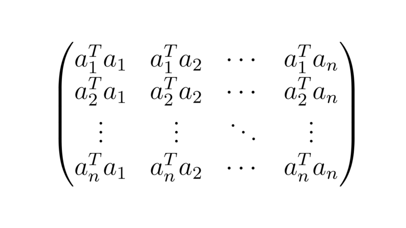
A common example of a symmetric matrix is the product $A^TA$, where $A$ is any $m\times n$ matrix. We use $A^TA$ when, for example, constructing the normal equations in least-squares problems. One way to see that it is symmetric for any matrix $A$ is to take the transpose of $A^TA$. $$(A^TA)^T = A^TA^{TT} = A^TA$$ The matrix is symmetric. But another way to see that $A^TA$ is symmetric is that for any rectangular matrix $A$ with columns $ a_1 ,\dotsc, a_n$, is to express the matrix product using the row-column rule for matrix multiplication.
\begin{align*}
A ^{T} A& =
\begin{pmatrix}
a_1 ^{T}
\\
a_2 ^{T}
\\
\vdots
\\
a_n ^{T}
\end{pmatrix}
\begin{pmatrix}
a_1 & a_2 & \cdots & a_n
\end{pmatrix}
=
\begin{pmatrix}
a_1 ^{T} a_1 & a_1 ^{T} a_2 & \cdots & a_1 ^{T} a_n
\\
a_2 ^T a_1 & a_2 ^{T} a_2 & \cdots & a_2 ^{T}a_n
\\
\vdots & \vdots & \ddots & \vdots
\\
a_n ^T a_1 & a_n ^{T} a_2 & \cdots & a_n ^{T}a_n
\end{pmatrix}
\end{align*}

Note that $a_i^Ta_j$ is the dot product between $a_i$ and $a_j$. And because dot products commute, in other words $$a_i^T a_j = a_i \cdot a_j = a_j \cdot a_i = a_j^Ta_i$$ $A^TA$ is symmetric.

One of the reasons that symmetric matrices are found in many algorithms is that they posses several properties that we can use to make useful or efficient calculations. In this section we investigate some of these properties that symmetric matrices have. In later sections of this chapter we will use these properties to develop and understand algorithms and their results.

Properties of Symmetric Matrices

In this section we give three theorems that characterize symmetric matrices.

Property 1) Symmetric Matrices Have Orthogonal Eigenspaces

The eigenspaces of symmetric matrices have a useful property that we can use when, for example, diagoanlizing a matrix.

If $ A$ is a symmetric matrix, with eigenvectors $ \vec v_1$ and $ \vec v_2$ corresponding to two distinct eigenvalues, then $\vec v_1$ and $\vec v_2$ are orthogonal.

More generally this theorem implies that eigenspaces associated to distinct eigenvalues are orthogonal subspaces.

Proof

Our approach will be to show that if $A$ is symmetric then any two of its eigenvectors $\vec v_1$ and $\vec v_2$ must be orthogonal when their corresponding eigenvalues $\lambda_1$ and $\lambda_2$ are not equal to each other.
\begin{align*} \lambda_1 \vec v_1 \cdot \vec v_2 &= A\vec v_1 \cdot \vec v_2 && \text{using } A\vec v_i = \lambda_i \vec v_i \\
&= (A\vec v_1)^T\vec v_2 && \text{using the definition of the dot product} \\
&= \vec v_1\,^TA^T\vec v_2 && \text{property of transpose of product}\\
&= \vec v_1\,^TA\vec v_2 && \text{given that } A = A^T\\
&= \vec v_1 \cdot A\vec v_2 && \text{again using the definition of the dot product}\\
&= \vec v_1 \cdot \lambda_2 \vec v_2 && \text{using } A\vec v_i = \lambda_i \vec v_i \\
&= \lambda_2 \vec v_1 \cdot \vec v_2
\end{align*}

Rearranging the equation yields

\begin{align*}
0 &= \lambda_2 \vec v_1 \cdot \vec v_2 – \lambda_1 \vec v_1 \cdot \vec v_2
= (\lambda_2 – \lambda_1) \vec v_1 \cdot \vec v_2
\end{align*}

But $\lambda_1 \ne \lambda_2$ so $\vec v_1 \cdot \vec v_2 = 0$. In other words, eigenvectors corresponding to distinct eigenvalues must be orthogonal. Our proof is complete.

2) The Eigenvalues of a Symmetric Matrix are Real

If $A$ is a real symmetric matrix then all eigenvalues of $A$ are real.

A proof of this result is in this post.

3) The Spectral Theorem

It turns out that every real symmetric matrix can always be diagonalized using an orthogonal matrix, which is a result of the spectral theorem:

An $ n \times n $ matrix $A$ is symmetric if and only if the matrix can be orthogonally diagonalized.

We will give a proof of the Spectral Theorem in a later post. But there are several important consequences of this theorem. All symmetric matrices can not only be diagonalized, but they can be diagonalized with an orthogonal matrix. Moreover, the only matrices that can be diagonalized orthogonally are symmetric, and that if a matrix can be diagonalized with an orthogonal matrix, then it is symmetric.

Examples

Example 1: Orthogonal Diagonalization of a $2\times 2$ Matrix

In this example we will diagonalize a matrix, $A$, using an orthogonal matrix, $P$.

$$A = \begin{pmatrix} 0 & -2\\ -2 & 3 \end{pmatrix}, \quad \lambda_1 = 4, \quad \lambda_2=-1$$

For eigenvalue $\lambda_1 = 4$ we have

$$A – \lambda_1 I = \begin{pmatrix} -4&-2\\-2&-1
\end{pmatrix} $$
A vector in the null space of $A – \lambda_1 I$ is the eigenvector
$$\vec v_1 =\begin{pmatrix}
1\\-2
\end{pmatrix}$$

A vector orthogonal to $\vec v_1$ is $$\vec v_2 = \begin{pmatrix}2\\1\end{pmatrix}$$ which must be an eigenvector for $\lambda_2$ because $A$ is symmetric.

Dividing each of the eigenvectors by their respective length, and then collecting these unit vectors into a single matrix, $P$, we obtain an orthogonal matrix. In other words,$P^{-1}P = PP^{-1} = I$. This convenient property gives us a convenient way to compute $P^{-1}$ should it be needed.

Placing the eigenvalues of $A$ in the order that matches the order used to create $P$, we obtain the factorization

$$A = PDP^T, \quad D = \begin{pmatrix} \lambda_1 & 0 \\ 0 & \lambda_2 \end{pmatrix}, \quad P = \frac{1}{\sqrt 5} \begin{pmatrix} 1&2\\-2& 1\end{pmatrix}$$

 

Example 2: Orthogonal Diagonalization of a $3\times3$ Matrix

In this example we will diagonalize a matrix, $A$, using an orthogonal matrix, $P$.

$$A = \begin{pmatrix} 0 & 0 & 1 \\ 0 & 1 & 0 \\ 1 & 0 & 0 \end{pmatrix} \quad \lambda = -1, 1$$

The eigenvalues of $A$ are given. For eigenvalue $\lambda_1 = -1$ we have

$$A – \lambda_1 I = \begin{pmatrix} 1&0&1\\0&2&0\\1&0&1
\end{pmatrix} \sim \begin{pmatrix} 1&0&1\\0&2&0\\1&0&1
\end{pmatrix}$$

A vector in the null space of $A – \lambda_1 I$ is the eigenvector

$$\vec v_1 =\begin{pmatrix}
1\\0\\-1
\end{pmatrix}$$

For eigenvalue $\lambda_2 = 1$ we have

$$A – \lambda_2 I = \begin{pmatrix} -1&0&1\\0&0&0\\1&0&-1
\end{pmatrix} \sim \begin{pmatrix} -1&0&1\\0&0&0\\0&0&0
\end{pmatrix}$$

By inspection, two vectors in the null space of $A – \lambda_2 I$ are

$$\vec v_2 = \begin{pmatrix} 0\\1\\0 \end{pmatrix}, \quad \vec v_3 = \begin{pmatrix} 1\\0\\1 \end{pmatrix}$$

There are many other choices that we could make but the above two vectors will suffice. Note that $\vec v_2$ and $\vec v_3$ happen to be orthogonal to each other. If they happened to not be orthogonal, one could use the Gram-Schmidt procedure to make them so.

Dividing each of the three eigenvectors by their respective length, and then collecting these unit vectors into a single matrix, $P$, we obtain an orthogonal matrix. This will give us a matrix whose inverse is equal to its transpose. In other words, $P$ is an orthogonal matrix, and $P^{-1}P = PP^{-1} = I$. This convenient property gives us a convenient way to compute $P^{-1}$ should it be needed.

Placing the eigenvalues of $A$ in the order that matches the order used to create $P$, we obtain the factorization

$$A = PDP^T, \quad D = \begin{pmatrix} \lambda_1 & 0 & 0 \\ 0 & \lambda_2 & 0 \\ 0 & 0 & \lambda_2 \end{pmatrix}, \quad P = \frac{1}{\sqrt 2} \begin{pmatrix} 1&0&1\\0&\sqrt2&0\\-1&0&1 \end{pmatrix}$$

Summary

In this post we explored how we might construct an orthogonal diagonalization of a symmetric matrix, $A = PDP^T$. Note that when a symmetric matrix has a repeated eigenvalue, Gram-Schmidt may be needed when eigenvalues are repeated to construct a full set of orthonormal eigenvectors that span $\mathbb R^n$. The theorems we introduced in this section gives us that when $A$ is symmetric, the eigenvalues of $A$ are real, eigenspaces of $A$ are mutually orthogonal, and $A$ can be diagonalized as $A = P D P ^{T}$.