Representing a Quadratic Form Using a Matrix

To motivate the use of linear algebra to study quadratic forms, consider the following problem. Does this inequality hold for all real values of $x$ and $y$?
\begin{equation*}
5x^2 + 8 y ^2 – 4 xy \geq 0
\end{equation*}

Were it not for the $-4xy$ term we could immediately tell that this statement is true. Because if the expression was $5x^2 + 8y^2 \geq 0$, we would more easily see that this can never be negative for any real values of $x$ and $y$. But could their sum ever be less than $4xy$? Because if it is, then $5x^2 + 8 y ^2 – 4xy$ would be negative and the inequality would not be true.

After introducing some theory and procedures we will circle back to this motivating problem. Our first step will be to draw a connection to quadratic forms, which allow us to study the above inequality in more general context.

Quadratic Forms

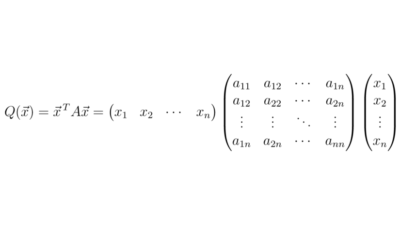
A quadratic form} is a function $ Q \;:\; \mathbb R ^{n} \to \mathbb R $, given by
\begin{equation*}
Q (\vec x ) = \vec x ^{\, T} A \vec x =
\begin{pmatrix}
x_1 & x _2 & \cdots & x_n
\end{pmatrix} \begin{pmatrix}
a_ {11} & a _{12} & \cdots & a _{1n}
\\
a _{12} & a _{22} & \cdots & a _{2n}
\\
\vdots & \vdots & \ddots & \vdots
\\
a _{1n} & a _{2n} & \cdots & a _{nn}
\end{pmatrix}
\begin{pmatrix}
x_1 \\ x _2\\ \vdots \\ x_n
\end{pmatrix}
\end{equation*}

Matrix $A$ is $n \times n$ and symmetric and $\vec x$ is a vector of variables. If we represent quadratic forms using a symmetric matrix, we can take advantage of their properties to solve problems like the one given at the start of this article. First we will explore a few example of quadratic forms so that we have a better understanding of what they are.

Example 1: Quadratic forms in $\mathbb R^2$

Consider the general quadratic form in two variables, $Q(x,y) =\vec x \, ^{T} A \vec x$, with $$A = \begin{pmatrix} a_{11} & a_{12} \\ a_{21} & a_{22} \end{pmatrix}, \quad \vec x = \begin{pmatrix}x\\y\end{pmatrix}$$
$A$ is symmetric, so we have $a_{12} = a_{21}$, and $$Q(x,y) = a_{11}x^2 + a_{22}y^2 + 2a_{12}xy$$

A particular example of a quadratic form familiar to many reading this section would be $$Q (x,y) = \begin{pmatrix} x & y \end{pmatrix} \begin{pmatrix} 1&0\\0&1 \end{pmatrix} \begin{pmatrix} x \\ y \end{pmatrix} = x^2 + y^2 $$ Setting $Q=r^2$ equal to a constant generates a set of points that create a circle with radius $r$. Two examples are shown in the diagram below.

\begin{center}
\begin{tikzpicture}[scale=0.6]

\draw[->,very thick] (-6.0,0) — (6.0,0) node [below] {$x$};
\draw[->,very thick] (0,-6.0) — (0,6.0) node [left] {$y$};
\draw[style=help lines,solid] (-6.2,-6.2) grid[step=2cm] (6.2,6.2);
\draw[DarkBlue] (0,2) node [left] {$2$};
\draw[DarkBlue] (2,0) node [below] {$2$};
\draw[DarkBlue] (0,-2) node [left] {$-2$};
\draw[DarkBlue] (-2,0) node [below] {$-2$};
\draw[DarkBlue] (0,4) node [left] {$4$};
\draw[DarkBlue] (4,0) node [below] {$4$};
\draw[DarkBlue] (0,-4) node [left] {$-4$};
\draw[DarkBlue] (-4,0) node [below] {$-4$};
\draw[rotate=0, DarkBlue, line width = 0.5mm] (0, 0) ellipse (1cm and 1cm);
\draw[DarkBlue] (3.2,0.9) node [above] {{\large $r^2=1=x^2+y^2$}};
\draw[rotate=0, DarkRed, line width = 0.5mm] (0, 0) ellipse (4cm and 4cm);
\draw[DarkRed] (3.2,4.1) node [above] {{\large $r^2=16=x^2+y^2$}};
% \draw[rotate=0, Black, line width = 0.3mm] (0, 0) ellipse (5cm and 5cm);
\end{tikzpicture}
\end{center}
Other choices of $Q$ and the entries in $A$ will create other curves in $\mathbb R^2$. For example, $Q = \vec x \, ^{T} A \vec x$ with
\begin{align*}
A &= \begin{pmatrix} 4 & -2 \\ -2 & 2 \end{pmatrix}
\end{align*}
generates a set of equations the form $Q = 4x^2 + 2y^2 – 4xy$, because
\begin{align*}
Q &= \begin{pmatrix} x & y \end{pmatrix}\begin{pmatrix} 4 & -2 \\ -2 & 2 \end{pmatrix} \begin{pmatrix} x \\ y \end{pmatrix} \\ &= \begin{pmatrix} x & y \end{pmatrix}\begin{pmatrix} 4x-2y \\ -2x+2y \end{pmatrix} \\ &= 4x^2 -2yx -2xy +2y^2 \\ &= 4x^2 + 2y^2 – 4xy
\end{align*}
If we set $Q=4$ we obtain the ellipse below.
\begin{center}
\begin{tikzpicture}[scale=1]

\draw[->,very thick] (-3.0,0) — (3.0,0) node [below] {$x$};
\draw[->,very thick] (0,-3.0) — (0,3.0) node [left] {$y$};
\draw[style=help lines,solid] (-3.2,-3.2) grid[step=1cm] (3.2,3.2);
\draw[DarkBlue] (0,2) node [left] {$2$};
\draw[DarkBlue] (2,0) node [below] {$2$};
\draw[DarkBlue] (0,-2) node [left] {$-2$};
\draw[DarkBlue] (-2,0) node [below] {$-2$};
\draw[rotate=58.3, black, line width = 0.5mm] (0, 0) ellipse (2.25cm and 0.9cm);
% \draw[DarkBlue] (3.2,0.9) node [above] {{\large $Q=4=4x^2+2y^2-4xy$}};
\end{tikzpicture}
\end{center}

Example 2: A Quadratic Form

In this example we express $Q = x^2 – 6 xy + 9 y ^2 $ in the form $Q = \vec x^T A \vec x$, where $\vec x \in \mathbb R^2$ and $A=A^T$. Placing coefficients of $x^2$ and $y^2$ on the main diagonal, and dividing coefficient of $xy$ by 2, we obtain
$$x^2 – 6 xy + 9 y ^2 = \begin{pmatrix} x & y \end{pmatrix}  \begin{pmatrix} 1&-3\\-3&9 \end{pmatrix} \begin{pmatrix} x \\ y \end{pmatrix}
$$
We can verify this result by multiplying $\vec x \, ^T A \vec x$.

Example 3: Quadratic Form in Three Variables

Write $Q$ in the form $\vec x^{T} A \vec x $ for $\vec x \in \mathbb R^3$.

$$Q (\vec x) = 5 x_1 ^2 – x_2 ^2 + 3 x_3 ^2 +6 x_1 x_3 – 12 x_2 x_3$$

Note that we can write $Q$ as

$$Q = 5 x_1 ^2 – x_2 ^2 + 3 x_3 ^2 +6 x_1 x_3 – 12 x_2 x_3 + 0 x_1x_2$$

Taking a similar approach to the previous exercise, we obtain

$$Q = \begin{pmatrix} x_1 & x_2 & x_3 \end{pmatrix} \begin{pmatrix} 5&0&3\\0&-1&-6\\3&-6&3 \end{pmatrix} \begin{pmatrix} x_1 \\ x_2 \\ x_3 \end{pmatrix}$$

Again, we can verify this result by multiplying $\vec x \, ^T A \vec x$.

The Principle Axes Theorem

One of the problems we will explore later in this course involves determining the points on a curve of the form $1 = \vec x \, ^TA\vec x$ that are closest or furthest from the origin. This particular problem will be aided with the Principal Axes Theorem.

If $A$ is a symmetric matrix then there exists an orthogonal change of variable $\vec x = P \vec y$ that transforms $\vec x^{\,T} A \vec x$ to $\vec y^{\,T} D \vec y$ with no cross-product terms.

The proof of this theorem relies on the fact that $A$ is a symmetric matrix and therefore can be diagonalized using an orthogonal matrix.

Proof

Given $Q(\vec x) = \vec x\,^T A\vec x$, where $\vec x \in \mathbb R^n$ is a variable vector and $A$ is a real $n\times n$ symmetric matrix. Then we can write $$A = PDP^T$$ where $P$ is an $n \times n$ orthogonal matrix. A change of variable} can be represented as $$\vec x = P\vec y, \quad \mathrm{or} \quad \vec y = P^{-1}\vec x$$ With this change of variable, the quadratic form $\vec x \,^T A\vec x$ becomes
\begin{align*}
Q = \vec x \,^T A\vec x &= (P\vec y)^T A (P\vec y) \\
&= \vec y\, ^T P^T A P\vec y \\
&= \vec y\, ^T D\vec y , \quad \text{using } A = PDP^T
\end{align*}

Thus, $Q$ is expressed without cross-product terms because $D$ is a diagonal matrix.

Example 4: Change of Variable

Consider the quadratic form $$Q = \vec x^{\,T} A \vec x, \quad A = \begin{pmatrix} 5 & 2 \\ 2 & 8 \end{pmatrix}$$ The eigenvalues and eigenvectors of $A$ are given below.

$$\lambda_1 = 9, \quad \lambda_2 = 4, \quad \vec v_1 = \begin{pmatrix} 2\\-1 \end{pmatrix}, \quad \vec v_2 = \begin{pmatrix} 1\\2 \end{pmatrix}$$

We will identify a change of variable that removes the cross-product term. Our change of variable is

$$\vec x = P \vec y, \quad P = \frac{1}{\sqrt5} \begin{pmatrix} 2&1\\-1&2 \end{pmatrix}$$

Using this change of variable,

$Q = \vec x\, ^TA\vec x = \vec y\, ^T D \vec y = 9y_1^2 + 4y_2^2$.

If, for example, we set $Q=1$, we obtain two curves in $\mathbb R^2$. One curve is $x_1x_2$-plane, the other in the $y_1y_2$-plane.

\begin{center}
\begin{tikzpicture}[scale=0.5]
\draw[->] (-3,0) — (3,0) node[right] {$x_1$};
\draw[->] (0,-3.5) — (0,3.5) node[right] {$x_2$};
\draw[rotate=35, black, line width = 0.4mm] (0, 0) ellipse (.75cm and 3cm);
\draw[style=help lines,solid] (-4.2,-4.2) grid[step=2cm] (4.2,4.2);
\draw[DarkBlue] (0,2) node [left] {$2$};
\draw[black] (0,-4.5) node [below] {$Q = 5x^2+4xy+8y^2= 1$};
\end{tikzpicture} \hspace{1cm}
\begin{tikzpicture}[scale=0.5]
\draw[->] (-3,0) — (3,0) node[right] {$y_1$};
\draw[->] (0,-3.5) — (0,3.5) node[right] {$y_2$};
\draw[rotate=0, Black, line width = 0.4mm] (0, 0) ellipse (1cm and 2cm);
\draw[style=help lines,solid] (-4.2,-4.2) grid[step=2cm] (4.2,4.2);
\draw[DarkBlue] (0,2) node [left] {$2$};
\draw[black] (0,-4.5) node [below] {$Q = 9y_1^2 + 4y_2^2 = 1 $ };
\end{tikzpicture}
\end{center}

Our change of variable can simplify our analysis. For example we can more easily identify points on the ellipse that are closest/furthest from the origin, and determine whether $Q$ can take on negative/positive values.

Example 5: Analyzing an Inequality Involving a Quadratic

We can now return to our motivating question from the start of this section. Does $x^2 – 6 xy + 9 y ^2 \geq 0$ hold for all $x,y$?

To answer this question we set $Q = 5x^2 – 4 xy + 8 y ^2$.

\begin{align*}
Q &= 5x^2 – 4 xy + 8 y ^2 = \vec x\, ^T A\vec x , \quad A = \begin{pmatrix} 5&-2\\-2&8 \end{pmatrix}
\end{align*}

The characteristic polynomial is $(\lambda-5)(\lambda – 8) -4 = (\lambda-9)(\lambda – 4)$. The eigenvalues therefore are $\lambda_1 = 4$ and $ \lambda_2 = 9$. Note that to quickly check that these numbers are, in fact, the eigenvalues of $A$, we could check whether $A – \lambda_1I$ and $A – \lambda_2I$ are singular.

Knowing the eigenvalues of $A$, we find that $$Q = \vec y \, ^T D \vec y = 4y_1^2 + 9 y_2^2$$

We see that $Q$ can be zero when $y_1=y_2=0$, but $Q$ is never negative. So the inequality is true.

Summary

We saw how we can express quadratic forms in the form $Q (\vec x ) = \vec x ^{\, T} A \vec x$, for $\vec x \in \mathbb R^n$. In this section we introduced a representation of quadratic forms with symmetric matrices. We saw how we can express quadratic forms in the form $Q (\vec x ) = \vec x ^{\, T} A \vec x$, for $\vec x \in \mathbb R^n$ without cross-product terms. We gave a change of variable to represent quadratic forms without cross-product terms and used the Principle Axis Theorem to investigate inequalities involving quadratic forms.

One of the reasons we are interested in quadratic forms is because they can be used to describe linear transforms. Consider the transform $\vec x \to A\vec x = \vec y$. The squared length of the vector $\vec y = A\vec x$ is a quadratic form.

$$\Vert \vec y \, \rVert= \lVert A \vec x \, \rVert^2 = (A\vec x) \cdot (A\vec x) = \vec x \, ^T A^TA \vec x$$ Because $A^TA$ is symmetric, we can use symmetric matrices and their properties to characterize linear transforms.