Applying Matrix Multiplication to 2D Computer Graphics

Linear transformations are often used in computer graphics to simulate the motion of an object. They can be computed using a matrix-vector product of the form $$T(\vec x) = A\vec x$$ where $\vec x$ is a vector that represents a point that is transformed to the vector $A\vec x$. The matrix-vector product $A\vec x$ is a transformation that acts on the vector $x$ to produce a new vector, $\vec b = A\vec x$. And if we set the function $T(\vec x)$ to be $$T(\vec x) = A\vec x = \vec b$$ then $T$ maps the vector $\vec x$ to vector $\vec b$. And the nature of the transform is described by matrix $A$.

Translations are a type of transformation needed in computer graphics. But translations are not a linear transformation because they do not leave the origin fixed. How might we use matrix multiplication in order to perform such transformations? In this section we answer this question by introducing homogeneous coordinates, which allow for more general transformations to be computed with linear algebra.

Homogeneous Coordinates

Each point $(x,y)$ in $\mathbb R^2$ can be identified with the homogeneous coordinate point $(x,y,1)$, on the plane in $\mathbb R^3$ that lies $1$ unit above the $xy$-plane.

For example, a translation of the form $(x,y) \to (x+h,y+k)$ is a transformation. The parameters $h$ and $k$ adjust the location of the point $(x,y)$ after the transformation. This transform can be represented as a matrix multiplication with homogeneous coordinates in the following way.

$$\begin{pmatrix} 1&0&h\\0&1&k\\0&0&1 \end{pmatrix} \begin{pmatrix} x\\y\\1 \end{pmatrix} = \begin{pmatrix} x+h\\y+k\\1 \end{pmatrix} $$

The first two entries can be extracted from the output of the transform to obtain the coordinate of the translated point.

The following examples demonstrate how homogeneous coordinates can be used to create more general transforms.

Example 1: A Composite Transform with a Translation

The transformation $T(\vec x)$ reflects points in $\mathbb R^2$ across the line $x_2 = x_1$ and then translates them by $2$ units in the $x_1$ direction and $3$ units in the $x_2$ direction. We can use homogeneous coordinates to construct a matrix $A$ so that $T = A\vec x$.

With homogeneous coordinates, any point $(x,y)$ can be represented by the vector $$\begin{pmatrix} x\\y\\1 \end{pmatrix}$$

Points in $\mathbb R^2$ can be reflected across the line $x_2 = x_1$ using the standard matrix

$$A_r = \begin{pmatrix} 0 & 1 \\ 1 & 0 \end{pmatrix}$$

With homogeneous coordinates our point is represented with a vector in $\mathbb R^3$, so we use the block matrix

$$A_1 = \begin{pmatrix} A_r & \textbf{0} \\ \textbf{0} & 1 \end{pmatrix} = \begin{pmatrix} 0 & 1 & 0 \\ 1 & 0 & 0 \\ 0 & 0 & 1 \end{pmatrix}$$

The symbol \textbf{0} denotes a matrix of zeroes. In this case, either a $1\times2$ matrix or a $2\times1$ matrix. Then the matrix-vector product below produces the needed transformation.

$$A_1 \vec x = \begin{pmatrix} 0 & 1 & 0 \\ 1 & 0 & 0 \\ 0 & 0 & 1 \end{pmatrix}\begin{pmatrix} x\\y\\1 \end{pmatrix}= \begin{pmatrix} y \\x\\1 \end{pmatrix}$$

Note that the $x_1$ and $x_2$ coordinates have been swapped, as required for the reflection through the line $x_2 = x_1$. The matrix below will perform the translation we need.

$$A_2 = \begin{pmatrix} 1 & 0 & 2 \\ 0 & 1 & 3 \\ 0 & 0 & 1 \end{pmatrix}$$

The product below will apply the translation, of $2$ units in the $x_1$ direction and $3$ units in the $x_2$ direction, to the reflected point.

$$T(\vec x) = A_2 (A_1 \vec x)= A_2 A_1 \vec x = \begin{pmatrix} 1 & 0 & 2 \\ 0 & 1 & 3 \\ 0 & 0 & 1 \end{pmatrix}\begin{pmatrix} y \\x\\1 \end{pmatrix} = \begin{pmatrix} y +2 \\x + 3\\1 \end{pmatrix} $$

Therefore, our standard matrix is
$$A = A_2A_1 = \begin{pmatrix} 1 & 0 & 2 \\ 0 & 1 & 3 \\ 0 & 0 & 1 \end{pmatrix} \begin{pmatrix} 0 & 1 & 0 \\ 1 & 0 & 0 \\ 0 & 0 & 1 \end{pmatrix} = \begin{pmatrix} 0 & 1 & 2 \\ 1 & 0 & 3 \\ 0 & 0 & 1 \end{pmatrix}$$

Example 2: Rotation About the Point (0,1)

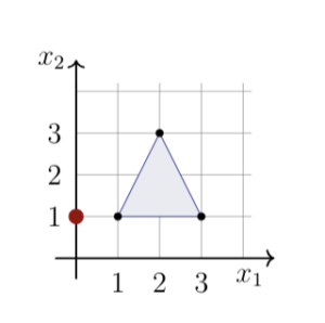
Triangle $S$ is determined by the points $(1,1), (2,4)$ and $(3,1)$. Transform $T$ rotates points by $\pi/2$ radians counterclockwise about the point $(0,1)$. Use matrix multiplication to determine the image of $S$ under $T$ and sketch $S$ and its image under $T$.

Suppose that we want to rotate our triangle by $\pi$ radians (or $180^{\circ}$) about the origin, $(0,0)$. A sketch of the triangle before and after the rotation is in the diagram below.

We need a way to calculate the locations of the points after the transformation. The rotation can be calculated by first representing each point by a vector in homogeneous coordinates, and then multiplying the vectors by a sequence of matrices that perform the needed transformation. The transformations will first shift the points in a way so that the rotation point is about the origin. We will then rotate about the origin by the desired about. And then we move the rotated points up by one unit to account for the initial translation.

Step 1: Shift Points Down by 1 Unit

In homogeneous coordinates our three points can be represented by the vectors below.

$$\vec a = \begin{pmatrix} 1\\1 \\1\end{pmatrix}, \quad \vec b = \begin{pmatrix} 2\\3\\1 \end{pmatrix} , \quad \vec c = \begin{pmatrix} 3\\1 \\1 \end{pmatrix} $$

Multiplying each vector by the matrix $$A_1 = \begin{pmatrix} 1 & 0 & 0 \\ 0 & 1 & -1 \\ 0 & 0 & 1 \end{pmatrix}$$
shifts the points down by one unit.

\begin{align*}
\vec a = \begin{pmatrix} 1\\1 \\1\end{pmatrix} \to & \ A_1 \vec a =\begin{pmatrix} 1 & 0 & 0 \\ 0 & 1 & -1 \\ 0 & 0 & 1 \end{pmatrix}\begin{pmatrix} 1\\1 \\1\end{pmatrix} = \begin{pmatrix} 1 \\ 0 \\ 1 \end{pmatrix} \\
\vec b = \begin{pmatrix} 2\\3 \\1\end{pmatrix} \to & \ A_1 \vec b =\begin{pmatrix} 1 & 0 & 0 \\ 0 & 1 & -1 \\ 0 & 0 & 1 \end{pmatrix}\begin{pmatrix} 1\\1 \\1\end{pmatrix} = \begin{pmatrix} 2 \\ 2 \\ 1 \end{pmatrix} \\
\vec c = \begin{pmatrix} 3\\1 \\1\end{pmatrix} \to & \ A_1 \vec c = \begin{pmatrix} 1 & 0 & 0 \\ 0 & 1 & -1 \\ 0 & 0 & 1 \end{pmatrix}\begin{pmatrix} 1\\1 \\1\end{pmatrix} = \begin{pmatrix} 3 \\ 0 \\ 1 \end{pmatrix}
\end{align*}

Notice how the only difference between the input and output vectors is that the second entry of the output vectors are one less than their corresponding entries in the input vectors. Our translated triangle and rotation point is shown below.

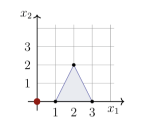
With this transform, the rotation point also moves down one unit, from $(0,1)$ to the origin $(0,0)$.

Step 2: Rotate About (0,0)

Rotating the translated points by $\pi/2$ radians about the origin can be calculated by multiplying the three vectors by the matrix

$$A_2 = \begin{pmatrix} 0 & -1 & 0 \\ 1 & 0 & 0 \\ 0 & 0 & 1\end{pmatrix}$$

This gives us three new points.

\begin{align*}
\vec a = \begin{pmatrix} 1\\1 \\1\end{pmatrix} \to & \ A_2A_1 \vec a =\begin{pmatrix} 0 & -1 & 0 \\ 1 & 0 & 0 \\ 0 & 0 & 1 \end{pmatrix} \begin{pmatrix} 1 \\ 0 \\ 1 \end{pmatrix} = \begin{pmatrix} 0 \\ 1 \\ 1 \end{pmatrix} \\
\vec b = \begin{pmatrix} 2\\3 \\1\end{pmatrix} \to & \ A_2A_1 \vec b =\begin{pmatrix} 0 & -1 & 0 \\ 1 & 0 & 0 \\ 0 & 0 & 1 \end{pmatrix} \begin{pmatrix} 2 \\ 2 \\ 1 \end{pmatrix} = \begin{pmatrix} -2 \\ 2 \\ 1 \end{pmatrix}\\
\vec c = \begin{pmatrix} 3\\1 \\1\end{pmatrix} \to & \ A_2A_1 \vec c =\begin{pmatrix} 0 & -1 & 0 \\ 1 & 0 & 0 \\ 0 & 0 & 1 \end{pmatrix} \begin{pmatrix} 3 \\ 0 \\ 1 \end{pmatrix} = \begin{pmatrix} 0 \\ 3 \\ 1 \end{pmatrix}
\end{align*}

Finally, to undo the initial translation that placed the rotation point at the origin, we need to translate our points up by one unit.

Step 3: Translate

Translating the data up by one unit can be accomplished by multiplying the three vectors by the matrix

$$A_3 = \begin{pmatrix} 1 & 0 & 0 \\ 0 & 1 & 1 \\ 0 & 0 & 1\end{pmatrix}$$

\This gives us three new points.

\begin{align*}
\vec a = \begin{pmatrix} 1\\1 \\1\end{pmatrix} \to & \ A_3A_2A_1 \vec a =\begin{pmatrix} 1 & 0 & 0 \\ 0 & 1 & 1 \\ 0 & 0 & 1 \end{pmatrix} \begin{pmatrix} 0 \\ 1 \\ 1 \end{pmatrix} = \begin{pmatrix} 0 \\ 2 \\1 \end{pmatrix}\\
\vec b = \begin{pmatrix} 2\\3 \\1\end{pmatrix} \to & \ A_3A_2A_1 \vec b =\begin{pmatrix} 1 & 0 & 0 \\ 0 & 1 & 1 \\ 0 & 0 & 1 \end{pmatrix} \begin{pmatrix} -2 \\ 2 \\ 1 \end{pmatrix} = \begin{pmatrix} -2\\3\\1 \end{pmatrix}\\
\vec c = \begin{pmatrix} 3\\1 \\1\end{pmatrix} \to & \ A_3A_2A_1 \vec c =\begin{pmatrix} 1 & 0 & 0 \\ 0 & 1 & 1 \\ 0 & 0 & 1 \end{pmatrix} \begin{pmatrix} 0 \\ 3 \\ 1 \end{pmatrix} = \begin{pmatrix} 0\\4\\1 \end{pmatrix}
\end{align*}

The standard matrix that performs a rotation by $\pi/2$ degrees about $(0,1)$ is the matrix $$A = A_3A_2A_1 = \begin{pmatrix} 1 & 0 & 0 \\ 0 & 1 & 1 \\ 0 & 0 & 1 \end{pmatrix} \begin{pmatrix} 0 & -1 & 0 \\ 1 & 0 & 0 \\ 0 & 0 & 1 \end{pmatrix} \begin{pmatrix} 1 & 0 & 0 \\ 0 & 1 & -1 \\ 0 & 0 & 1 \end{pmatrix} = \begin{pmatrix} 0 & -1 & 1 \\ 1 & 0 & 1 \\ 0 & 0 & 1 \end{pmatrix} $$ The result can be verified by calculating $A\vec a$, $A\vec b$, or $A \vec c$.

Our rotated triangle is shown below.

Example 3: A Reflection Through The Line $x_2 = x_1 + 3$

Let’s determine the $3\times3$ standard matrix, $A$, that uses homogeneous coordinates to reflect points in $\mathbb R^2$ across the line $x_2 = x_1 + 3$. And also confirm that our results are correct by calculating $T(\vec x) = A\vec x$ for any point $\vec x$ that uses homogeneous coordinates.

The standard matrix $A$ will be the product of three matrices that translate and reflect points using homogeneous coordinates. The first matrix will translate points so that the line about which we are reflecting passes through the origin. We can use

$$A_1 = \begin{pmatrix} 1 & 0 & 0 \\ 0 & 1 & -3 \\ 0 & 0 & 1 \end{pmatrix}$$

This matrix will shift points down three units so that the line $x_2 = x_1 + 3$ will pass through the origin. The second matrix will reflect points through the shifted line, which is $x_2= x_1$. Recall that the matrix

$$\begin{pmatrix} 0 & 1 \\ 1 & 0 \end{pmatrix}$$

will reflect vectors in $\mathbb R^2$ through the line $x_2 = x_1$. This is because any point with coordinates $(x_1,x_2)$ can be represented with the vector

$$\vec x = \begin{pmatrix} x_1 \\ x_2 \end{pmatrix}$$

and

$$\begin{pmatrix} 0 & 1 \\ 1 & 0 \end{pmatrix}\begin{pmatrix}x_1 \\ x_2 \end{pmatrix} = \begin{pmatrix} x_2 \\ x_1 \end{pmatrix}$$

The point $(x_1,x_2)$ is mapped to $(x_2,x_1)$, which is a reflection through the line $x_2 = x_1$. The standard matrix for this transformation in homogeneous coordinates is

$$A_2 = \begin{pmatrix} 0 & 1 & 0 \\ 1 & 0 & 0 \\ 0 & 0 & 1 \end{pmatrix}$$

Our final transformation shifts points back up by three units to undo the initial translation.

$$A_3 = \begin{pmatrix} 0 & 1 & 0 \\ 1 & 0 & 3 \\ 0 & 0 & 1 \end{pmatrix}$$

The standard matrix for the transformation that reflects points in $\mathbb R^2$ across the line $x_2 = x_1 + 3$ is

$$A = A_3A_2A_1 = \begin{pmatrix} 0 & 1 & 0 \\ 1 & 0 & 3 \\ 0 & 0 & 1 \end{pmatrix}\begin{pmatrix} 0 & 1 & 0 \\ 1 & 0 & 0 \\ 0 & 0 & 1 \end{pmatrix}\begin{pmatrix} 1 & 0 & 0 \\ 0 & 1 & -3 \\ 0 & 0 & 1 \end{pmatrix} = \begin{pmatrix} 0 & 1 & -3 \\ 1 & 0 & 3 \\ 0 & 0 & 1 \end{pmatrix}$$

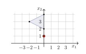
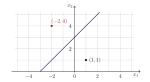
We can check whether our work is correct by transforming any point $(x_1,x_2)$ with the above standard matrix. For example, the point $(1,1)$ is transformed by calculating

$$T(\vec x) = A\vec x = \begin{pmatrix} 0 & 1 & -3 \\ 1 & 0 & 3 \\ 0 & 0 & 1 \end{pmatrix}\begin{pmatrix}1\\1\\1 \end{pmatrix} = \begin{pmatrix} -2 \\ 4 \\1 \end{pmatrix}$$

The reflected point is $(-2,4)$. The line of reflection, initial point, and the reflected point are shown below.

The Data Matrix

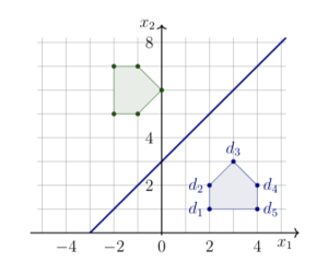
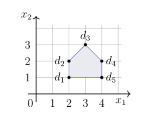
The examples in this section have only involved a small number points that need to be transformed. For problems involving many points, it may be more convenient to represent the points in what we refer to as a \Emph{data matrix}. For example, the shape in the figure below is determined by five points, or vertices, $d_1, d_2, \ldots , d_5$. Their respective homogeneous coordinates can be stored in the columns of a matrix, $D$.

$$D = \begin{pmatrix} \vec d_1 & \vec d_2& \vec d_3& \vec d_4& \vec d_5 \end{pmatrix} = \begin{pmatrix} 2&2&3&4&4\\1&2&3&2&1\\1&1&1&1&1 \end{pmatrix}$$

For our purposes, the order in which the points are placed into $D$ is arbitrary.

In the previous examples we applied a transform with a matrix-vector multiplication. With a data matrix we can use a similar approach. Recall that the product of two matrices $A$ and $D$, is defined as $$AD = A\begin{pmatrix} \vec d_1 & \vec d_2 & \cdots & \vec d_p\end{pmatrix} = \begin{pmatrix} A\vec d_1 & A\vec d_2 & \cdots & A\vec d_p\end{pmatrix}$$ where $\vec d_1, \vec d_2, \cdots , \vec d_p$ are the columns of $D$. In other words, can perform the transformation on our data by computing $AD$, which transforms each column independently of the others.

For example, applying the transform in the previous example will reflect our shape through the line $x_2 = x_1 + 3$. The transformation is found by computing

$$AD = \begin{pmatrix} 0 & 1 & -3 \\ 1 & 0 & 3 \\ 0 & 0 & 1 \end{pmatrix}\begin{pmatrix} 2&2&3&4&4\\1&2&3&2&1\\1&1&1&1&1 \end{pmatrix} = \begin{pmatrix} -2&-1&0&-1&-2\\5&5&6&7&7\\1&1&1&1&1\end{pmatrix}$$

Extracting the first two entries of each column of the result gives us the transformed points (green), as shown in the figure below.